Graphein RNA Graph Construction Tutorial
In this notebook we construct graphs of RNA structures. The workflow we follow is similar to the other data modalities. The desired edge constructions are passed as a list of functions to the construction function.


[1]:
# Install Graphein if necessary
# !pip install graphein
Constructing 2D RNA Graphs
The inputs we require are a sequence (optional) and a dotbracket specification of the secondary structure.
[5]:
from rich import inspect
import matplotlib.pyplot as plt

from typing import List, Callable
import networkx as nx
import graphein.rna as gr
Construction with a Dotbracket
Graph construction is handled by the `construct_graph() <https://graphein.ai/modules/graphein.rna.html#graphein.rna.graphs.construct_graph>`__ function.
Dotbrackets are strings composed of, funnily enough, dots : "." and brackets: "(" / ")" (in their simplest form) that denote RNA secondary structures. Each character in the string represents a base, open brackets indicate a base is paired to a base ahead of it in the sequence and, conversely, closed brackets denote that a base is paired a preceding position.
[6]:
inspect(gr.construct_graph)
╭────────────────────── <function construct_graph at 0x7f7789a26700> ───────────────────────╮
│ def construct_graph(dotbracket: Union[str, NoneType] = None, sequence: Union[str,         │
│ NoneType] = None, bprna_id: Union[str, NoneType] = None, use_nussinov: bool = False,      │
│ config: Union[graphein.rna.config.RNAGraphConfig, NoneType] = None, pdb_path: Union[str,  │
│ NoneType] = None, pdb_code: Union[str, NoneType] = None, chain_selection: str = 'all',    │
│ rna_df_processing_funcs: Union[List[Callable], NoneType] = None, edge_construction_funcs: │
│ Union[List[Callable], NoneType] = None, edge_annotation_funcs: Union[List[Callable],      │
│ NoneType] = None, node_annotation_funcs: Union[List[Callable], NoneType] = None,          │
│ graph_annotation_funcs: Union[List[Callable], NoneType] = None) ->                        │
│ networkx.classes.graph.Graph:                                                             │
│                                                                                           │
│ 35 attribute(s) not shown. Run inspect(inspect) for options.                              │
╰───────────────────────────────────────────────────────────────────────────────────────────╯
[7]:
edge_funcs_1: List[Callable] = [
    gr.add_base_pairing_interactions,
    gr.add_phosphodiester_bonds,
    gr.add_pseudoknots,
]
edge_funcs_2: List[Callable] = [gr.add_all_dotbracket_edges]

g = gr.construct_graph(
    "......((((((......[[[))))))......]]]....",
    sequence=None,
    edge_construction_funcs=edge_funcs_1,
)
nx.draw(g)

gr.plot_rna_graph(g, layout=nx.layout.spring_layout)
No sequence data found in graph. Skipping base type labelling.
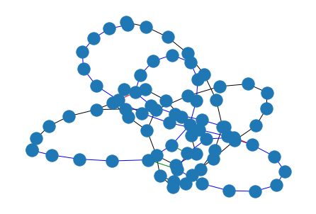
Construction with a dotbracket and sequence
[11]:
g = gr.construct_graph(
    sequence="CGUCUUAAACUCAUCACCGUGUGGAGCUGCGACCCUUCCCUAGAUUCGAAGACGAG",
    dotbracket="((((((...(((..(((...))))))...(((..((.....))..)))))))))..",
    edge_construction_funcs=edge_funcs_1,
)
plt.subplot(121)
gr.plot_rna_graph(g, layout=nx.layout.spring_layout)
plt.subplot(122)
gr.plot_rna_graph(g, layout=nx.layout.circular_layout) # We can use any nx layout we wish
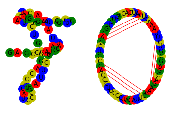
Using the Nussinov Algorithm to predict Secondary Structure with only a Sequence
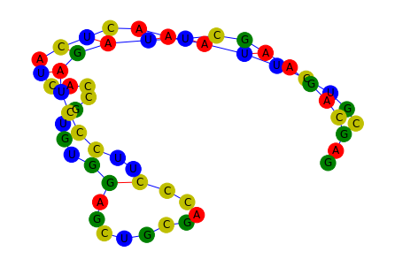
The Nussinov Algorithm is a DP-based approach to predict the secondary structure of RNA molecules. This is useful in the scenario where you have an RNA sequence but no known/determined secondary structure.
Description
(From the wiki article)
Scoring
We score a solution by counting the total number of paired bases. Thus, attempting to maximize the score maximizes the total number of bonds between bases.
Motivation
Consider an RNA sequence \(S\) whose elements are taken from the set \(\{A,U,C,G\}\). Let us imagine we have an optimal solution to the subproblem of folding \(S_{i}\) to \(S_{j-1}\), and an optimal solution for folding \(S_{u}\) to \(S_{v}\) $ i:nbsphinx-math:leq `u:nbsphinx-math:leq v:nbsphinx-math:leq j-1$. Now, to align :math:`S_{i} to \(S_{j}\), we have two options:
Leave \(S_{j}\) unpaired, and keep the structure of \(S_{i}\) to \(S_{j-1}\). The score for this alignment will be equal to the score of the alignment of \(S_{i}\) to \(S_{j-1}\), as no new base pairs were created.
Pair \(S_{j}\) with \(S_{k}\), where \(i\leq k<j\). The score for this alignment will be the score of the base pairing, plus the score of the best alignment of \(S_{i}\) to \(S_{k-1}\) and \(S_{k+1}\) to \(S_{j-1}\).
Caveat Emptors
The algorithm does not account for the 3D structure of RNA
The algorithm does not predict pseudoknots
It does not account for a minimum stem loop size.
[12]:
# NBVAL_SKIP
g = gr.construct_graph(
    sequence="CGUCUUAAACUCAUCACCGUGUGGAGCUGCGACCCUUCCCUAGAUUCGAAGACGAG",
    dotbracket=None,
    edge_construction_funcs=edge_funcs_1,
    use_nussinov=True
)
gr.plot_rna_graph(g, layout=nx.layout.spring_layout)
inspect(g.graph)
╭───────────────────────────────── <class 'dict'> ──────────────────────────────────╮
│ dict() -> new empty dictionary                                                    │
│ dict(mapping) -> new dictionary initialized from a mapping object's               │
│     (key, value) pairs                                                            │
│ dict(iterable) -> new dictionary initialized as if via:                           │
│     d = {}                                                                        │
│     for k, v in iterable:                                                         │
│         d[k] = v                                                                  │
│ dict(**kwargs) -> new dictionary initialized with the name=value pairs            │
│     in the keyword argument list.  For example:  dict(one=1, two=2)               │
│                                                                                   │
│ ╭───────────────────────────────────────────────────────────────────────────────╮ │
│ │ {                                                                             │ │
│ │ │   'dotbracket': '((((((((..((.(.(..(.(.((..........)..)))))))))..))))))..', │ │
│ │ │   'sequence': 'CGUCUUAAACUCAUCACCGUGUGGAGCUGCGACCCUUCCCUAGAUUCGAAGACGAG'    │ │
│ │ }                                                                             │ │
│ ╰───────────────────────────────────────────────────────────────────────────────╯ │
│                                                                                   │
│ 30 attribute(s) not shown. Run inspect(inspect) for options.                      │
╰───────────────────────────────────────────────────────────────────────────────────╯
Constructing 3D Graphs of RNA Structures
Similar to Protein Structures, we can construct 3D graphs of RNA structures in the PDB using `graphein.rna.construct_graph() <https://graphein.ai/modules/graphein.rna.html#graphein.rna.graphs.construct_graph>`__.
Config
[26]:
config = gr.RNAGraphConfig()
inspect(config)
╭────────────────────── <class 'graphein.rna.config.RNAGraphConfig'> ───────────────────────╮
│ Config Object for RNA Structure Graph Construction.                                       │
│                                                                                           │
│ ╭───────────────────────────────────────────────────────────────────────────────────────╮ │
│ │ RNAGraphConfig(granularity='rna_atom', verbose=False,                                 │ │
│ │ edge_construction_functions=[<function add_atomic_edges at 0x7f78fa9da5e0>],          │ │
│ │ rna_df_processing_functions=None, node_metadata_functions=None,                       │ │
│ │ edge_metadata_functions=None, graph_metadata_functions=None)                          │ │
│ ╰───────────────────────────────────────────────────────────────────────────────────────╯ │
│                                                                                           │
│ edge_construction_functions = [<function add_atomic_edges at 0x7f78fa9da5e0>]             │
│     edge_metadata_functions = None                                                        │
│                 granularity = 'rna_atom'                                                  │
│    graph_metadata_functions = None                                                        │
│     node_metadata_functions = None                                                        │
│ rna_df_processing_functions = None                                                        │
│                     verbose = False                                                       │
╰───────────────────────────────────────────────────────────────────────────────────────────╯
[27]:
g = gr.construct_graph(pdb_code="2jyf", config=config)
gr.plotly_rna_structure_graph(g, colour_nodes_by="residue_name")
Data type cannot be displayed: application/vnd.plotly.v1+json
[28]:
inspect(g.graph)
╭───────────────────────────────────── <class 'dict'> ──────────────────────────────────────╮ │ dict() -> new empty dictionary │ │ dict(mapping) -> new dictionary initialized from a mapping object's │ │ (key, value) pairs │ │ dict(iterable) -> new dictionary initialized as if via: │ │ d = {} │ │ for k, v in iterable: │ │ d[k] = v │ │ dict(**kwargs) -> new dictionary initialized with the name=value pairs │ │ in the keyword argument list. For example: dict(one=1, two=2) │ │ │ │ ╭───────────────────────────────────────────────────────────────────────────────────────╮ │ │ │ { │ │ │ │ │ 'name': '2jyf', │ │ │ │ │ 'pdb_id': '2jyf', │ │ │ │ │ 'chain_ids': ['A', 'B'], │ │ │ │ │ 'pdb_df': record_name atom_number blank_1 atom_name alt_loc residue_name │ │ │ │ blank_2 \ │ │ │ │ 0 ATOM 1 O5' G │ │ │ │ 1 ATOM 2 C5' G │ │ │ │ 2 ATOM 3 C4' G │ │ │ │ 3 ATOM 4 O4' G │ │ │ │ 4 ATOM 5 C3' G │ │ │ │ ... ... ... ... ... ... ... ... │ │ │ │ 1831 ATOM 2750 N3 U │ │ │ │ 1832 ATOM 2751 C4 U │ │ │ │ 1833 ATOM 2752 O4 U │ │ │ │ 1834 ATOM 2753 C5 U │ │ │ │ 1835 ATOM 2754 C6 U │ │ │ │ │ │ │ │ │ │ chain_id residue_number insertion ... y_coord z_coord occupancy \ │ │ │ │ 0 A 1 ... -37.668 9.239 1.0 │ │ │ │ 1 A 1 ... -38.206 8.391 1.0 │ │ │ │ 2 A 1 ... -38.940 7.196 1.0 │ │ │ │ 3 A 1 ... -40.138 7.644 1.0 │ │ │ │ 4 A 1 ... -38.116 6.432 1.0 │ │ │ │ ... ... ... ... ... ... ... ... │ │ │ │ 1831 B 86 ... 35.469 18.786 1.0 │ │ │ │ 1832 B 86 ... 34.331 19.486 1.0 │ │ │ │ 1833 B 86 ... 33.400 19.625 1.0 │ │ │ │ 1834 B 86 ... 34.366 20.002 1.0 │ │ │ │ 1835 B 86 ... 35.442 19.793 1.0 │ │ │ │ │ │ │ │ │ │ b_factor blank_4 segment_id element_symbol charge line_idx \ │ │ │ │ 0 1.0 O NaN 130 │ │ │ │ 1 1.0 C NaN 131 │ │ │ │ 2 1.0 C NaN 132 │ │ │ │ 3 1.0 O NaN 133 │ │ │ │ 4 1.0 C NaN 134 │ │ │ │ ... ... ... ... ... ... ... │ │ │ │ 1831 1.0 N NaN 2879 │ │ │ │ 1832 1.0 C NaN 2880 │ │ │ │ 1833 1.0 O NaN 2881 │ │ │ │ 1834 1.0 C NaN 2882 │ │ │ │ 1835 1.0 C NaN 2883 │ │ │ │ │ │ │ │ │ │ │ │ │ │ node_id │ │ │ │ 0 A:G:1:1:O5' │ │ │ │ 1 A:G:1:2:C5' │ │ │ │ 2 A:G:1:3:C4' │ │ │ │ 3 A:G:1:4:O4' │ │ │ │ 4 A:G:1:5:C3' │ │ │ │ ... ... │ │ │ │ 1831 B:U:86:2750:N3 │ │ │ │ 1832 B:U:86:2751:C4 │ │ │ │ 1833 B:U:86:2752:O4 │ │ │ │ 1834 B:U:86:2753:C5 │ │ │ │ 1835 B:U:86:2754:C6 │ │ │ │ │ │ │ │ [1836 rows x 22 columns], │ │ │ │ │ 'raw_pdb_df': record_name atom_number blank_1 atom_name alt_loc │ │ │ │ residue_name blank_2 \ │ │ │ │ 0 ATOM 1 O5' G │ │ │ │ 1 ATOM 2 C5' G │ │ │ │ 2 ATOM 3 C4' G │ │ │ │ 3 ATOM 4 O4' G │ │ │ │ 4 ATOM 5 C3' G │ │ │ │ ... ... ... ... ... ... ... ... │ │ │ │ 27635 ATOM 2761 HO2' U │ │ │ │ 27636 ATOM 2762 H1' U │ │ │ │ 27637 ATOM 2763 H3 U │ │ │ │ 27638 ATOM 2764 H5 U │ │ │ │ 27639 ATOM 2765 H6 U │ │ │ │ │ │ │ │ │ │ chain_id residue_number insertion ... y_coord z_coord occupancy \ │ │ │ │ 0 A 1 ... -37.668 9.239 1.0 │ │ │ │ 1 A 1 ... -38.206 8.391 1.0 │ │ │ │ 2 A 1 ... -38.940 7.196 1.0 │ │ │ │ 3 A 1 ... -40.138 7.644 1.0 │ │ │ │ 4 A 1 ... -38.116 6.432 1.0 │ │ │ │ ... ... ... ... ... ... ... ... │ │ │ │ 27635 B 86 ... 40.905 10.613 1.0 │ │ │ │ 27636 B 86 ... 39.008 11.258 1.0 │ │ │ │ 27637 B 86 ... 38.303 15.344 1.0 │ │ │ │ 27638 B 86 ... 37.987 16.026 1.0 │ │ │ │ 27639 B 86 ... 38.644 13.718 1.0 │ │ │ │ │ │ │ │ │ │ b_factor blank_4 segment_id element_symbol charge line_idx \ │ │ │ │ 0 1.0 O NaN 130 │ │ │ │ 1 1.0 C NaN 131 │ │ │ │ 2 1.0 C NaN 132 │ │ │ │ 3 1.0 O NaN 133 │ │ │ │ 4 1.0 C NaN 134 │ │ │ │ ... ... ... ... ... ... ... │ │ │ │ 27635 1.0 H NaN 27802 │ │ │ │ 27636 1.0 H NaN 27803 │ │ │ │ 27637 1.0 H NaN 27804 │ │ │ │ 27638 1.0 H NaN 27805 │ │ │ │ 27639 1.0 H NaN 27806 │ │ │ │ │ │ │ │ │ │ │ │ │ │ │ │ node_id │ │ │ │ 0 A:G:1:1:O5' │ │ │ │ 1 A:G:1:2:C5' │ │ │ │ 2 A:G:1:3:C4' │ │ │ │ 3 A:G:1:4:O4' │ │ │ │ 4 A:G:1:5:C3' │ │ │ │ ... ... │ │ │ │ 27635 B:U:86:2761:HO2' │ │ │ │ 27636 B:U:86:2762:H1' │ │ │ │ 27637 B:U:86:2763:H3 │ │ │ │ 27638 B:U:86:2764:H5 │ │ │ │ 27639 B:U:86:2765:H6 │ │ │ │ │ │ │ │ [27640 rows x 22 columns], │ │ │ │ │ 'rgroup_df': record_name atom_number blank_1 atom_name alt_loc residue_name │ │ │ │ blank_2 \ │ │ │ │ 0 ATOM 1 O5' G │ │ │ │ 1 ATOM 2 C5' G │ │ │ │ 2 ATOM 3 C4' G │ │ │ │ 3 ATOM 4 O4' G │ │ │ │ 4 ATOM 5 C3' G │ │ │ │ ... ... ... ... ... ... ... ... │ │ │ │ 2759 ATOM 2761 HO2' U │ │ │ │ 2760 ATOM 2762 H1' U │ │ │ │ 2761 ATOM 2763 H3 U │ │ │ │ 2762 ATOM 2764 H5 U │ │ │ │ 2763 ATOM 2765 H6 U │ │ │ │ │ │ │ │ │ │ chain_id residue_number insertion ... y_coord z_coord occupancy \ │ │ │ │ 0 A 1 ... -37.668 9.239 1.0 │ │ │ │ 1 A 1 ... -38.206 8.391 1.0 │ │ │ │ 2 A 1 ... -38.940 7.196 1.0 │ │ │ │ 3 A 1 ... -40.138 7.644 1.0 │ │ │ │ 4 A 1 ... -38.116 6.432 1.0 │ │ │ │ ... ... ... ... ... ... ... ... │ │ │ │ 2759 B 86 ... 39.771 18.792 1.0 │ │ │ │ 2760 B 86 ... 38.212 17.955 1.0 │ │ │ │ 2761 B 86 ... 35.491 18.406 1.0 │ │ │ │ 2762 B 86 ... 33.518 20.570 1.0 │ │ │ │ 2763 B 86 ... 35.443 20.194 1.0 │ │ │ │ │ │ │ │ │ │ b_factor blank_4 segment_id element_symbol charge line_idx \ │ │ │ │ 0 1.0 O NaN 130 │ │ │ │ 1 1.0 C NaN 131 │ │ │ │ 2 1.0 C NaN 132 │ │ │ │ 3 1.0 O NaN 133 │ │ │ │ 4 1.0 C NaN 134 │ │ │ │ ... ... ... ... ... ... ... │ │ │ │ 2759 1.0 H NaN 2890 │ │ │ │ 2760 1.0 H NaN 2891 │ │ │ │ 2761 1.0 H NaN 2892 │ │ │ │ 2762 1.0 H NaN 2893 │ │ │ │ 2763 1.0 H NaN 2894 │ │ │ │ │ │ │ │ │ │ │ │ │ │ node_id │ │ │ │ 0 A:G:1:1:O5' │ │ │ │ 1 A:G:1:2:C5' │ │ │ │ 2 A:G:1:3:C4' │ │ │ │ 3 A:G:1:4:O4' │ │ │ │ 4 A:G:1:5:C3' │ │ │ │ ... ... │ │ │ │ 2759 B:U:86:2761:HO2' │ │ │ │ 2760 B:U:86:2762:H1' │ │ │ │ 2761 B:U:86:2763:H3 │ │ │ │ 2762 B:U:86:2764:H5 │ │ │ │ 2763 B:U:86:2765:H6 │ │ │ │ │ │ │ │ [2764 rows x 22 columns], │ │ │ │ │ 'coords': array([[ 6.291, -37.668, 9.239], │ │ │ │ │ [ 7.307, -38.206, 8.391], │ │ │ │ │ [ 6.703, -38.94 , 7.196], │ │ │ │ │ ..., │ │ │ │ │ [ 2.641, 33.4 , 19.625], │ │ │ │ │ [ 4.782, 34.366, 20.002], │ │ │ │ │ [ 5.579, 35.442, 19.793]]), │ │ │ │ │ 'node_type': 'rna_atom', │ │ │ │ │ 'sequence_A': 'GGGGGGGGGGGGGGGGGGGGGGGGGGGGGGGGGGGGGGGGGGGGGGGGGGGGGGGGGGGG'+858, │ │ │ │ │ 'sequence_B': 'GGGGGGGGGGGGGGGGGGGGGGGGGGGGGGGGGGGGGGGGGGGGGGGGGGGGGGGGGGGG'+858, │ │ │ │ │ ... +2 │ │ │ │ } │ │ │ ╰───────────────────────────────────────────────────────────────────────────────────────╯ │ │ │ │ 30 attribute(s) not shown. Run inspect(inspect) for options. │ ╰───────────────────────────────────────────────────────────────────────────────────────────╯
[15]:
# Quickly grab the first node so we can see the contained metadata
nodes = list(g.nodes(data=True))
inspect(nodes[0])
╭────────────────────── <class 'tuple'> ───────────────────────╮
│ Built-in immutable sequence.                                 │
│                                                              │
│ ╭──────────────────────────────────────────────────────────╮ │
│ │ (                                                        │ │
│ │ │   "A:G:1:1:O5'",                                       │ │
│ │ │   {                                                    │ │
│ │ │   │   'chain_id': 'A',                                 │ │
│ │ │   │   'residue_name': 'G',                             │ │
│ │ │   │   'residue_number': 1,                             │ │
│ │ │   │   'atom_type': "O5'",                              │ │
│ │ │   │   'element_symbol': 'O',                           │ │
│ │ │   │   'coords': array([  6.291, -37.668,   9.239]),    │ │
│ │ │   │   'b_factor': 1.0,                                 │ │
│ │ │   │   'atomic_radius': 0.67                            │ │
│ │ │   }                                                    │ │
│ │ )                                                        │ │
│ ╰──────────────────────────────────────────────────────────╯ │
│                                                              │
│ 31 attribute(s) not shown. Run inspect(inspect) for options. │
╰──────────────────────────────────────────────────────────────╯
Nodes are given unique string identifiers. This is a little more involved than a protein structure where we can (almost!) uniquely identify a given residue by CHAIN:RESIDUE:SEA_POSITION and a given atom by CHAIN:RESIDUE:SEQ_POSITION:ATOM_NAME
For RNA, we adopt a CHAIN:BASE:SEQ_POSITION:ATOM_NUMBER:ATOM_NAME. The inclusion of the atom number in the identifier is required due to the possibility of the presence of complementary strand (which is not treated as another chain in the graph). This can be seen clearly in our example (two complementary strands form each chain)
[16]:
gr.plotly_rna_structure_graph(g, colour_nodes_by="chain")
Data type cannot be displayed: application/vnd.plotly.v1+json
Alternative Edge Construction Schemes
Most of the spatial edge constructions functions used in the protein API should apply to RNA. Here we construct a graph using both edges based on K-NN connectivity (using \(k=5\)) and spatial edges, joining two nodes if they are within \(4 \AA\) of one another.
[17]:
from functools import partial

config = gr.RNAGraphConfig(
    edge_construction_functions=[
        partial(gr.add_k_nn_edges, k=5, long_interaction_threshold=-1),
        partial(gr.add_distance_threshold, threshold=3, long_interaction_threshold=-1),
        ]
)

g = gr.construct_graph(pdb_code="2jyf", config=config)
gr.plotly_rna_structure_graph(g, colour_nodes_by="residue_name", node_size_min=1)
Data type cannot be displayed: application/vnd.plotly.v1+json
Extracting Subgraphs from 3D RNA Structure Graphs
We can use graphein’s selection capabilities to extract subgraphs of RNA structures. These functions behave analogously to the `subgraph extraction for proteins <>`__ (see tutorial for more details). However, there are some protein-specific selections and some RNA-specific selections so there is not perfect overlap.
The available methods for RNA structures are:
`extract_subgraph_from_node_list()<https://graphein.ai/modules/graphein.rna.html#graphein.rna.subgraphs.extract_subgraph_from_node_list>`__`extract_subgraph_from_backbone()<https://graphein.ai/modules/graphein.rna.html#graphein.rna.subgraphs.extract_subgraph_from_backbone>`__`extract_subgraph_from_bases()<https://graphein.ai/modules/graphein.rna.html#graphein.rna.subgraphs.extract_subgraph_from_bases>`__`extract_subgraph_from_phosphoric_acid()<https://graphein.ai/modules/graphein.rna.html#graphein.rna.subgraphs.extract_subgraph_from_phosphoric_acid>`__`extract_subgraph_from_ribose()<https://graphein.ai/modules/graphein.rna.html#graphein.rna.subgraphs.extract_subgraph_from_ribose>`__`extract_subgraph_from_point()<https://graphein.ai/modules/graphein.rna.html#graphein.rna.subgraphs.extract_subgraph_from_point>`__`extract_subgraph_from_atom_types()<https://graphein.ai/modules/graphein.rna.html#graphein.rna.subgraphs.extract_subgraph_from_atom_types>`__`extract_subgraph_from_residue_types()<https://graphein.ai/modules/graphein.rna.html#graphein.rna.subgraphs.extract_subgraph_from_residue_types>`__`extract_subgraph_from_chains()<https://graphein.ai/modules/graphein.rna.html#graphein.rna.subgraphs.extract_subgraph_from_chains>`__`extract_subgraph_by_sequence_position()<https://graphein.ai/modules/graphein.rna.html#graphein.rna.subgraphs.extract_subgraph_by_sequence_position>`__`extract_subgraph_by_bond_type()<https://graphein.ai/modules/graphein.rna.html#graphein.rna.subgraphs.extract_subgraph_by_bond_type>`__`extract_k_hop_subgraph()<https://graphein.ai/modules/graphein.rna.html#graphein.rna.subgraphs.extract_k_hop_subgraph>`__
We illustrate a few examples below
Extracting Backbone Subgraphs
[18]:
config = gr.RNAGraphConfig()
g = gr.construct_graph(pdb_code="2jyf", config=config)

s_g = gr.extract_subgraph_from_backbone(g)
gr.plotly_rna_structure_graph(s_g, colour_nodes_by="seq_position")
Data type cannot be displayed: application/vnd.plotly.v1+json
Extracting Base Subgraphs
We can similarly extract a subgraph using only atoms contained in the nitrogenous bases.
[19]:
config = gr.RNAGraphConfig()
g = gr.construct_graph(pdb_code="2jyf", config=config)

s_g = gr.extract_subgraph_from_bases(g)
gr.plotly_rna_structure_graph(s_g, colour_nodes_by="seq_position")
Data type cannot be displayed: application/vnd.plotly.v1+json
Extracting Chain Subgraphs
We can extract subgraphs containing only selections of chains
[20]:
config = gr.RNAGraphConfig()
g = gr.construct_graph(pdb_code="2jyf", config=config)

s_g = gr.extract_subgraph_from_chains(g, chains=["B"])
gr.plotly_rna_structure_graph(s_g, colour_nodes_by="chain_id")
Data type cannot be displayed: application/vnd.plotly.v1+json
Extracting Subgraphs Based on Sequence Position
We can extract subgraphs based on the position in the nucleotide sequence.
[21]:
config = gr.RNAGraphConfig()
g = gr.construct_graph(pdb_code="2jyf", config=config)

s_g = gr.extract_subgraph_by_sequence_position(g, sequence_positions=[1, 3, 5, 10])
gr.plotly_rna_structure_graph(s_g, colour_nodes_by="residue_number")
Data type cannot be displayed: application/vnd.plotly.v1+json
A note on using subgraphs in ML
As can be seen, we will often obtain a graph with many components (depending on the initial graph construction and the selection method). Using the previous subgraph as an example, we obtain 4 connected components. It is advisable to add new edges if you wish to obtain a graph with one connected component.
In this example we extract a subgraph containing only atoms that are part of the nitrogenous bases. We then add add K-nn edges on top of their covalent structure to result in a connected graph.
[22]:
import networkx as nx #TODO remove
print(f"Number of components: {nx.number_connected_components(s_g)}")
Number of components: 4
[23]:
config = gr.RNAGraphConfig()
g = gr.construct_graph(pdb_code="2jyf", config=config)

# Extract subgraph from bases
s_g = gr.extract_subgraph_by_sequence_position(g, sequence_positions=[1, 3, 5, 10])

# Add edges to subgraph
gr.add_k_nn_edges(s_g, k=22, long_interaction_threshold=-1)

print(f"Number of components: {nx.number_connected_components(s_g)}")
gr.plotly_rna_structure_graph(s_g, colour_nodes_by="seq_position")
Number of components: 1
Data type cannot be displayed: application/vnd.plotly.v1+json
We can save the selections to a PDB file for use elsewhere in the bioinformatics universe :)
N.B. This will not preserve connectivity and metadata
[24]:
from graphein.protein.utils import save_graph_to_pdb
save_graph_to_pdb(s_g, "selection.pdb")
/home/atj39/anaconda3/envs/graphein/lib/python3.8/site-packages/biopandas/pdb/pandas_pdb.py:554: UserWarning:

Column node_id is not an expected column and will be skipped.
[25]:
# Reading it back in
g = gr.construct_graph(path="selection.pdb")
gr.plotly_rna_structure_graph(g, colour_nodes_by="seq_position")
Data type cannot be displayed: application/vnd.plotly.v1+json